Lecture Summary: Loops

Repetition

The Natural Numbers (A Refresher on Induction)

Counting is a repetitive task. We count: 0, 1, 2, 3, 4, 5, ... It is not possible enumerate all numbers (because there are infinitely many of them). Instead, we use rules to describe the entirety of natural numbers. Finitely many rules are sufficient to describe infinitely many objects. Define,

0 is a natural number
If n is a natural number, then the successor n' is a natural number
For any predicate Φ, if

Φ is true, and
Φ is true implies Φ(n') is true, for any natural number n, then Φ(n) is true for all natural numbers n.

The natural numbers are defined by induction, starting from 0, specifying successors (a, b). To prove properties Φ about natural numbers we use complete induction (c)

Addition of Natural Numbers (A Refresher on Recursion)

Knowing the rule how to enumerate natural numbers, we could enumerate their sums 0 + 0 = 0, 1 + 0 = 1, 2 + 0 = 2, ...... A better way to describe addition is to exploit the inductive definition of natural numbers. We define “+” recursively 0 + x = x n' + x = (n + x)' where n' is the successor of n. Using the recursive definition, we can calculate 3 + 1 = (2 + 1)' = (1 + 1)'' = (0 + 1)''' = 1''' = 4 To prove properties about “+” we use complete induction. Claim: m + n ≥ m Proof by induction on m.

Base case (x = 0): 0 + n = n ≥ 0 because all natural numbers are at least 0. Inductive step: Assume induction hypothesis m + n ≥ m, hence m' + n = (m + n)' ≥ m' because x ≥ y implies x' ≥ y' and induction hypothesis. End of proof

Addition of Natural Numbers (A Refresher on Iteration)

Instead of recursion we can use iteration to add two natural numbers m and n. k = n i = m while i > 0 k = k + 1 i = i - 1 where k contains the sum of m and n when the program terminates. Calculation of a sum is not as straightforward as in the recursive case. It’s not immediately clear how we could prove m + n = k ≥ m In general, iteration is more intricate.

The reasoning about iteration is complicated by the use of mutable variables. However, without mutable variables iteration is not useful!

We prefer recursion for specification – it is easy to comprehend. Often iteration (and mutable variables) are more efficient. So, we prefer to use it for implementation.

Addition of Natural Numbers (A Refresher on Tail Recursion)

Any iteration, such as, k = n i = m while i > 0 k = k + 1 i = i - 1 can be written as a tail-recursive program (where the recursive call always comes last) (k, i) = *add*(k, i) where *add*(k, i) = if i > 0 *add*(k + 1, i - 1) else (k, i) Note that, the call to add comes after k + 1 and i - 1. Therefore, add is tail recursive. Tail-recursive functions and the corresponding iterative programs are essentially the same. As a consequence, we can use induction to reason about iteration as well. But we do not need to take a detour via a tail-recursive function. We can do it directly using (inductive) invariants.

Counting Down by Iteration

Example: Iteratively Counting Down to Zero

The following program counts down to zero.

 1
 2
 3
 4
 5
 6
 7
 8
 9
10
11
12
13


var n: Z = randomInt()
assume(n >= 0)


while (n > 0) {
  
  
  n = n - 1
  
}


assert(n == 0)

Let’s see what we know to be true at different locations in the program. By reasoning about the program we want to establish that the assertion n == 0 holds at the end of the program.

Tracing Facts by Looking Forward

At the beginning of the loop body the loop condition must be true.

 1
 2
 3
 4
 5
 6
 7
 8
 9
10
11
12
13


var n: Z = randomInt()
assume(n >= 0)


while (n > 0) {
  // deduce n > 0
  
  n = n - 1
  
}


assert(n == 0)

This fact must be true because the loop condition has just been evaluated to true when the loop body is entered.

After the loop the negation of the loop condition must be true.

 1
 2
 3
 4
 5
 6
 7
 8
 9
10
11
12
13


var n: Z = randomInt()
assume(n >= 0)


while (n > 0) {
  // deduce n > 0
  
  n = n - 1
  
}
// deduce n <= 0

assert(n == 0)

This fact must be true because the loop condition has just been evaluated to false when the loop is exited.

From the assumption we can also determine that n >= 0 must be true before the loop.

 1
 2
 3
 4
 5
 6
 7
 8
 9
10
11
12
13


var n: Z = randomInt()
assume(n >= 0)

// deduce n >= 0
while (n > 0) {
  // deduce n > 0
  
  n = n - 1
  
}
// deduce n <= 0

assert(n == 0)

We know this because of the assumption we make. That’s all we can deduce forward. Let’s consider what we can find out “looking back” from the assertion.

Tracing Facts by Looking Backward

We need to show that n == 0.

 1
 2
 3
 4
 5
 6
 7
 8
 9
10
11
12
13


var n: Z = randomInt()
assume(n >= 0)

// deduce n >= 0
while (n > 0) {
  // deduce n > 0
  
  n = n - 1
  
}
// deduce n <= 0

assert(n == 0)

We already know that n <= 0 after the loop. If we knew also that n >= 0 we could deduce n == 0 Let’s add a conjecture n >= 0

We only conjecture that n >= 0! should be true, but we don’t know this yet.

 1
 2
 3
 4
 5
 6
 7
 8
 9
10
11
12
13


var n: Z = randomInt()
assume(n >= 0)

// deduce n >= 0
while (n > 0) {
  // deduce n > 0
  
  n = n - 1
  
}
// deduce n <= 0
// deduce n >= 0 ?
assert(n == 0)

If the loop was never entered, then it would be true because n >= 0 is true before the loop (by assumption). If the loop was entered, n >= 0 would have to be true at the end of the body just before the loop could be exited.

We only conjecture that n >= 0 should be true, but we don’t know this yet.

 1
 2
 3
 4
 5
 6
 7
 8
 9
10
11
12
13


var n: Z = randomInt()
assume(n >= 0)

// deduce n >= 0
while (n > 0) {
  // deduce n > 0
  
  n = n - 1
  
}
// deduce n <= 0
// deduce n >= 0 ?
assert(n == 0)

We conjecture that n >= 0 should be true at the end of the body.

 1
 2
 3
 4
 5
 6
 7
 8
 9
10
11
12
13


var n: Z = randomInt()
assume(n >= 0)

// deduce n >= 0
while (n > 0) {
  // deduce n > 0
  
  n = n - 1
  // deduce n >= 0 ?
}
// deduce n <= 0
// deduce n >= 0 ?
assert(n == 0)

Continuing backwards, let’s have a look at the assignment n = n - 1. If n >= 0 was true after the assignment, then n - 1 >= 0 would have to have been true before the assignment. Where n - 1 >= 0 is n >= 0 with n replaced by n - 1.

Where n - 1 >= 0 is n >= 0 with n replaced by n - 1. The fact n - 1 >= 0 obtains n >= 0 pretending the assignment never took place. Now, n - 1 >= 0 is equivalent to n > 0 by algebra. Hence, it’s true and all conjectures are proved.

Tracing Facts by Looking Forward (Again)

We now have the following program with all currently known facts.

 1
 2
 3
 4
 5
 6
 7
 8
 9
10
11
12
13


var n: Z = randomInt()
assume(n >= 0)

// deduce n >= 0
while (n > 0) {
  // deduce n > 0
  
  n = n - 1
  // deduce n >= 0
}
// deduce n <= 0
// deduce n >= 0
assert(n == 0)

These facts are sufficient to show that the assertion is true. Having all these facts, there is one more fact that we can deduce forward now. We know that n > 0 is true before the loop and at the end of the loop body. Thus, it must be true at the beginning of the loop body.

Tracing Facts Summary

Now we have:

 1
 2
 3
 4
 5
 6
 7
 8
 9
10
11
12
13


var n: Z = randomInt()
assume(n >= 0)

// deduce n >= 0
while (n > 0) {
  // deduce n > 0
  // deduce n >= 0
  n = n - 1
  // deduce n >= 0
}
// deduce n <= 0
// deduce n >= 0
assert(n == 0)

In fact, we are allowed to assume that the fact n >= 0 at the beginning of the loop. Together with the loop condition n > 0 it forms the inductive hypothesis for the loop. The fact n >= 0 is central for the proof. It is called an (inductive) invariant for the loop.

We mention it explicitly.

 1
 2
 3
 4
 5
 6
 7
 8
 9
10
11
12
13


var n: Z = randomInt()
assume(n >= 0)

// deduce n >= 0
while (n > 0) {
  // invariant n >= 0
  // deduce n > 0
  n = n - 1
  // deduce n >= 0
}
// deduce n <= 0
// deduce n >= 0
assert(n == 0)

We also document which variables change in the loop body by way of a frame. This describes which variables may be modified, supporting understanding. And it describes which variables are renamed in the loop.

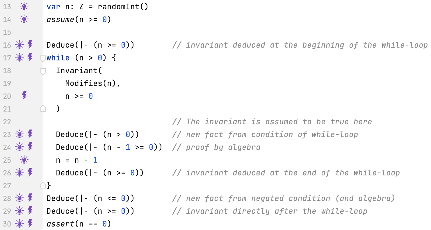
Finally, we have all information needed for reasoning about the loop.

 1
 2
 3
 4
 5
 6
 7
 8
 9
10
11
12
13


var n: Z = randomInt()
assume(n >= 0)

// deduce n >= 0
while (n > 0) {
  // invariant n >= 0, modifies n
  // deduce n > 0
  n = n - 1
  // deduce n >= 0
}
// deduce n <= 0
// deduce n >= 0
assert(n == 0)

Recall how we have used a combination of forward and backward reasoning to reduce the gap between what we know and what we have to prove. Now we can describe a rule for proving while-loops correct.

Invariant Rule for Proving Loops Correct

The following program counts down to zero.

 1
 2
 3
 4
 5
 6
 7
 8
 9
10
11


// ... deduce I
while (C) {
  // invariant I
  //   modifies "variables modified in body"
  // deduce C
  // deduce I
  body
  // ... deduce I
}
// deduce !C
// deduce I

We have to prove that the invariant I is true before the loop and at the end of the loop body. The modifies clause must specify at least those variables modified in the body. It describes what is allowed to change. Remark. Candidates for invariants can often be found by reasoning backwards.

Example: Iteratively Counting Down to Zero in Logika

Counting_Down_Slang The invariant is specified by.

1
2
3
4


Invariant(
  Modifies(n),
  n >= 0
)

Termination

In this course we mostly focus on reasoning about facts we can deduce should a program terminate This is called partial correctness.

In addition to the above, we can prove that a program terminates. This is called total correctness

Let’s have a brief look at termination. We return to it later in the course.

Termination of a Loop

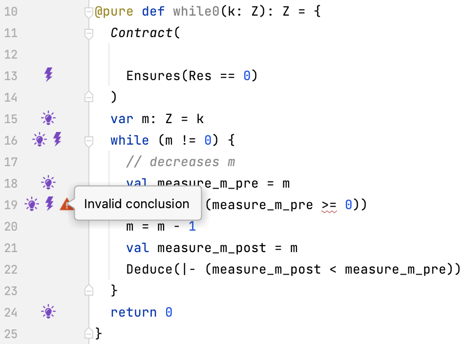
Let’s encapsulate the iterative counting-down program in a function

 1
 2
 3
 4
 5
 6
 7
 8
 9
10
11
12
13
14
15
16


@pure def while0(k: Z): Z = {
  Contract(
    
    Ensures(Res == 0)
  )
  var m: Z = k
  while (m != 0) {
    
    
    
    m = m - 1
    
    
  }
  return 0
}

We can prove about this function that, should the loop terminate, then it returns 0. What happens if the function is called with the argument -3, that is, while0(-3) ?

Measuring Termination of a Loop

If we could show that the always terminates, we would be certain the function returns 0.

 1
 2
 3
 4
 5
 6
 7
 8
 9
10
11
12
13
14
15
16


@pure def while0(k: Z): Z = {
  Contract(
    
    Ensures(Res == 0)
  )
  var m: Z = k
  while (m != 0) {
    
    
    
    m = m - 1
    
    
  }
  return 0
}

If no progress can be observed the program might not terminate

To observe progress we define measure

The measure must decrease during each loop iteration and not cross a given minimum (just like the progress bar)

This guarantees termination

Let’s introduce a measure for the loop

We need a method for verifying progress, like observing a progress bar. Observed progress: [insert progress bar] while0(10) returns 0.

A Measure for the Iterative Count-Down Function

The loop decreases m in each iteration, so m appears a good measure.

 1
 2
 3
 4
 5
 6
 7
 8
 9
10
11
12
13
14
15
16


@pure def while0(k: Z): Z = {
  Contract(
    
    Ensures(Res == 0)
  )
  var m: Z = k
  while (m != 0) {
    // decreases m
    
    
    m = m - 1
    
    
  }
  return 0
}

We have to prove that m decreases, but not beyond a given minimum, say, 0.

Let’s introduce auxiliary variable for the observation.

 1
 2
 3
 4
 5
 6
 7
 8
 9
10
11
12
13
14
15
16


@pure def while0(k: Z): Z = {
  Contract(
    
    Ensures(Res == 0)
  )
  var m: Z = k
  while (m != 0) {
    // decreases m
    val measure_m_pre = m
    
    m = m - 1
    val measure_m_post = m
    
  }
  return 0
}

Variable measure_m_pre observes the measure at the beginning of the loop body. Variable measure_m_post observes the measure at the end of the loop body.

We can deduce that the measure decreases.

 1
 2
 3
 4
 5
 6
 7
 8
 9
10
11
12
13
14
15
16


@pure def while0(k: Z): Z = {
  Contract(
    
    Ensures(Res == 0)
  )
  var m: Z = k
  while (m != 0) {
    // decreases m
    val measure_m_pre = m
    
    m = m - 1
    val measure_m_post = m
    Deduce(|- (measure_m_post < measure_m_pre))
  }
  return 0
}

The fact measure_m_post < measure_m_pre is true at the end of the loop body.

We cannot deduce that the measure does not cross the minimum 0.

 1
 2
 3
 4
 5
 6
 7
 8
 9
10
11
12
13
14
15
16


@pure def while0(k: Z): Z = {
  Contract(
    
    Ensures(Res == 0)
  )
  var m: Z = k
  while (m != 0) {
    // decreases m
    val measure_m_pre = m
    Deduce(|- (measure_m_pre >= 0))
    m = m - 1
    val measure_m_post = m
    Deduce(|- (measure_m_post < measure_m_pre))
  }
  return 0
}

Logika_Termination_Loop

Having instrumented the program with the measure, we can use Logika for proof support. In fact, we do not know whether m >= 0 when the loop is first entered.

A pre-condition can constrain k such that m is at least 0.

 1
 2
 3
 4
 5
 6
 7
 8
 9
10
11
12
13
14
15
16


@pure def while0(k: Z): Z = {
  Contract(
    Requires(k >= 0),
    Ensures(Res == 0)
  )
  var m: Z = k
  while (m != 0) {
    // decreases m
    val measure_m_pre = m
    Deduce(|- (measure_m_pre >= 0))
    m = m - 1
    val measure_m_post = m
    Deduce(|- (measure_m_post < measure_m_pre))
  }
  return 0
}

Logika_proved

A Recursive Count-Down Function

Similarly, to iteratively counting down, we can count down recursively.

 1
 2
 3
 4
 5
 6
 7
 8
 9
10
11
12
13
14
15
16


@pure def count0(k: Z): Z = {
  Contract(
  
    Ensures(Res == 0)
  )
  
  
  
  if (k == 0) {
    return k
  } else {
    
    
    return count0(k - 1)
  }
}

We need a measure on a function parameters that is bounded below when the function is entered and decreased at each recursive call.

A Measure for the Recursive Count-Down Function

Parameter k seems like a good candidate for a measure (It’s the only candidate, of course).

 1
 2
 3
 4
 5
 6
 7
 8
 9
10
11
12
13
14
15
16


@pure def count0(k: Z): Z = {
  Contract(
  
    Ensures(Res == 0)
  )
  // decreases k
  
  
  if (k == 0) {
    return k
  } else {
    
    
    return count0(k - 1)
  }
}

Let’s introduce two auxiliary variables measure_k_entry and `measure_k_call to observe progress.

The function instrumented for observation of the measure:

 1
 2
 3
 4
 5
 6
 7
 8
 9
10
11
12
13
14
15
16


@pure def count0(k: Z): Z = {
  Contract(
  
    Ensures(Res == 0)
  )
  // decreases k
  val measure_k_entry: Z = k       // value of the measure on entry
  
  if (k == 0) {
    return k
  } else {
    val measure_k_call: Z = k - 1  // value of the measure in the recursive call
    
    return count0(k - 1)
  }
}

Variable measure_k_entry observes the measure when the function is entered. Variable measure_k_call observes the measure in the recursive call.

We can deduce that the measure is deceased at the recursive call.

 1
 2
 3
 4
 5
 6
 7
 8
 9
10
11
12
13
14
15
16


@pure def count0(k: Z): Z = {
  Contract(
  
    Ensures(Res == 0)
  )
  // decreases k
  val measure_k_entry: Z = k
  
  if (k == 0) {
    return k
  } else {
    val measure_k_call: Z = k - 1
    Deduce(|- (measure_k_call < measure_k_entry))
    return count0(k - 1)
  }
}

Indeed, we have measure_k_call < measure_k_entry.

We cannot deduce that the measure is bounded below by 0.

 1
 2
 3
 4
 5
 6
 7
 8
 9
10
11
12
13
14
15
16


@pure def count0(k: Z): Z = {
  Contract(
  
    Ensures(Res == 0)
  )
  // decreases k
  val measure_k_entry: Z = k
  Deduce(|- (k >= 0))
  if (k == 0) {
    return k
  } else {
    val measure_k_call: Z = k - 1
    Deduce(|- (measure_k_call < measure_k_entry))
    return count0(k - 1)
  }
}

Logika_Termination_Recursion

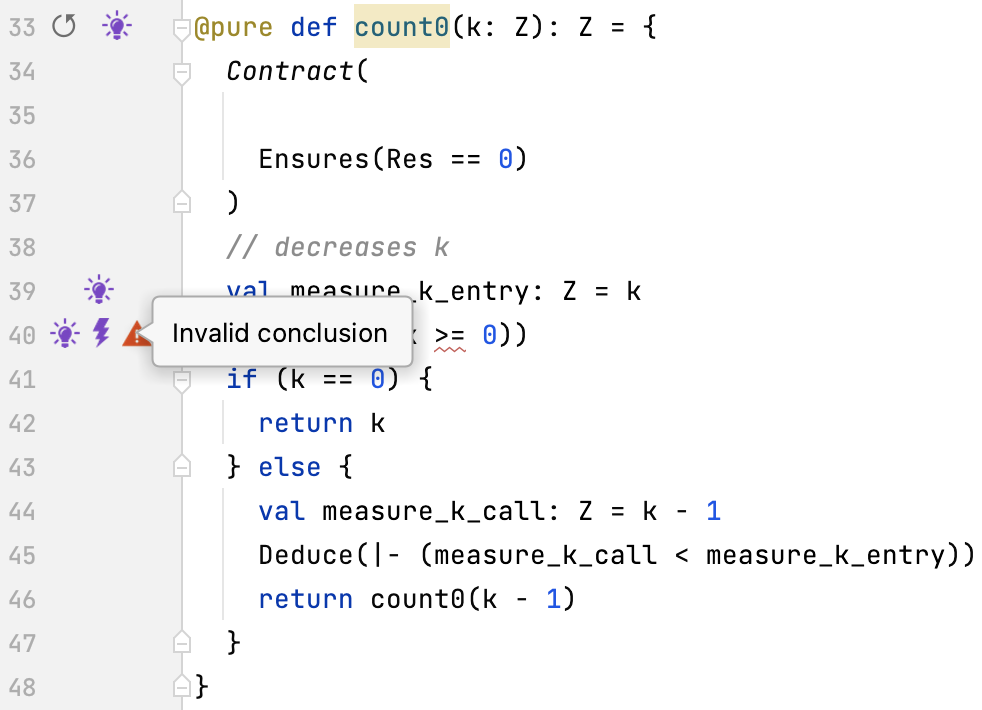
When the function is entered, there is no guarantee that k would be at least0. As in the case of the iterative version, this can be achieve by means of a pre-condition.

With the precondition added, the termination proof succeeds.

 1
 2
 3
 4
 5
 6
 7
 8
 9
10
11
12
13
14
15
16


@pure def count0(k: Z): Z = {
  Contract(
    Requires(k >= 0),
    Ensures(Res == 0)
  )
  // decreases k
  val measure_k_entry: Z = k
  Deduce(|- (k >= 0))
  if (k == 0) {
    return k
  } else {
    val measure_k_call: Z = k - 1
    Deduce(|- (measure_k_call < measure_k_entry))
    return count0(k - 1)
  }
}

Logika_proved

The Factorial Function

Next we consider a more complete example.

We begin with a (mathematical) specification of the factorial function. Subsequently, we provide a recursive implementation (that is easy to understand). Finally, we implement an iterative version of the factorial function and prove that it is correct with respect to the recursive implementation and thus with respect to the (mathematical) specification.

This approach permits us to move from a description of a program that is easy to understand to one that is efficient to execute. Often, the first recursive implementation is composed of a number of mathematical specifications and because of it’s simplicity we consider the recursive implementation a specification itself.

What we consider a specification is a matter of perspective.

Mathematical Specification of the Factorial

The factorial of a natural number n is usually specified based on their inductive definition.

1
2
3
4


@strictpure def fac_rec_spec(n: Z): Z = n match {
  case 0 => 1
  case m => m * fac_rec_spec(m - 1)
}

The definition is recursive matching the inductive definition of the natural numbers. The base case (n == 0) returns an expression. The inductive case (n > 0) contains the recursive call (with n - 1). Remark. We use the type of integer numbers for simplicity.

Aside. The attribute @strictpure limits the constructs that can be used in a function. We use it to obtain “mathematical” definitions. The Scala expression.

1
2
3
4
5


e match {
  case p1 => r1
  ...
  case pn => r1
}

matches expression e with the first possible pi and returns the corresponding ri.

Induction Rules the Factorial

We formulate inductive rules for proving properties about the factorial.

 1
 2
 3
 4
 5
 6
 7
 8
 9
10
11
12
13
14


// Base case
@pure def fac_rec_spec_0() {
  Contract(
    Ensures(fac_rec_spec(0) == 1)
  )
}

// Inductive case
@pure def fac_rec_spec_step(n: Z) {
  Contract(
    Requires(n > 0),
    Ensures(fac_rec_spec(n) == n * fac_rec_spec(n - 1))
  )
}

Using the recursive definition of fac_rec_spec and the inductive numbers these are straightforward to derive. Logika “knows” these rules.

Recursive Implementation of the Factorial

Following the mathematical definition very closely, we implement the factorial recursively.

 1
 2
 3
 4
 5
 6
 7
 8
 9
10
11


@pure def fac_rec(n: Z): Z = {
  Contract(
    Requires(n >= 0),
    Ensures(Res == fac_rec_spec(n))
  )
  if (n == 0) {
    return 1
  } else {
    return n * fac_rec(n - 1)
  }
}

Because the implementation is so close to the mathematical definition, Logika can prove it without further information. Specifications should be as “obvious” as possible. Let’s implement fac_rec iteratively.

Iterative Implementation of the Factorial

The iterative implementation fac_rec(see post-condition).

 1
 2
 3
 4
 5
 6
 7
 8
 9
10
11
12
13
14
15
16
17
18
19
20
21
22
23
24
25


@pure def fac_it(n: Z): Z = {
  Contract(
    Requires(n >= 0),
    Ensures(Res == fac_rec(n))
  )
  var x: Z = 1
  var m: Z = 0;
  while (m < n) {
    Invariant(
      Modifies(x, m),
      (x == fac_rec(m)),                        // invariant maintained until m == n,
      (m <= n),                                 // yielding post-condition x == fac_rec(n).
      (m >= 0)                                  // m >= 0 needed for pre-condition of fac_rec
    )
    Deduce(|- (m < n))                          // new fact from condition (forward)
    Deduce(|- (x * (m + 1) == fac_rec(m + 1)))  // proved fact (backward conjecture)
    m = m + 1
    Deduce(|- (x * m == fac_rec(m)))            // proved fact (backward conjecture)
    x = x * m
    Deduce(|- (x == fac_rec(m)))                // proved fact (backward conjecture)
  }
  Deduce(|- (m >= n))                           // new fact from negation of condition (forward).
  Deduce(|- (m <= n))                           // replace n by loop index variable m to obtain
  return x                                      // invariant x == fac_rec(m) from post-condition
}

Recursive Implementation of the Factorial

We have proved:

1
2
3
4
5
6


@pure def facimp(n: Z) {
  Contract(
    Requires(n >= 0),
    Ensures(fac_it(n) == fac_rec(n))
  )
}

that is, given n >= 0, the recursive specification and the iterative implementation are inter-replaceable.

We have implemented the factorial function correctly.

Exercise 1

Prove that fac_rec terminates. Prove that fac_it terminates.

The Fibonacci Function

Mathematical Specification of the Fibonacci Number

The fibonacci number for n is specified as follows.

1
2
3
4
5


@strictpure def fib_rec_spec(n: Z): Z = n match {
  case 0 => 0
  case 1 => 1
  case m => fib_rec_spec(m - 1) + fib_rec_spec(m - 2)
}

Exercise 2

State the inductive rules for fib_rec_spec (There are three of them!)
Implement the recursive function fib_rec computing the fibonacci number
Prove that fib_rec terminates using Logika

Exercise 3

 1
 2
 3
 4
 5
 6
 7
 8
 9
10
11
12
13
14
15
16
17
18
19
20
21
22
23
24
25
26


@pure def fib_it(n: Z): Z = {
  Contract(
    Requires(n >= 0),
    Ensures(Res == fib_rec(n))
  )
  if (n == 0) {
    return 0
  } else if (n == 1) {
    return 1
  } else {
    var x: Z = 0
    var y: Z = 1
    var m: Z = 1;
    while (m < n) {
      Invariant(
        Modifies(x, y, m),
        (x == fib_rec(m - 1)),
        (y == fib_rec(m)),
        (m <= n),
        (m >= 0)
      )
      ...
    }
    return y
  }
}

Complete the implementation of the iterative version fib_it

Do not introduce any additional variable
Hint: Look at the previous example of in-place number swapping

Prove your implementation correct using Logika
Prove that your implementation terminates using Logika

Slang Examples

Count Int Loop Rec

 1
 2
 3
 4
 5
 6
 7
 8
 9
10
11
12
13
14
15
16
17
18
19
20
21
22
23
24
25
26
27
28
29
30
31
32
33
34
35
36
37
38
39
40
41
42
43
44
45
46
47
48
49
50
51
52
53
54
55
56
57
58
59
60


// #Sireum #Logika
import org.sireum._

var p: Z = randomInt()
assume(p >= 0)

while (p > 0) {
  p = p - 1
  assert(true)
}
assert(p == 0)

var n: Z = randomInt()
assume(n >= 0)

Deduce(|- (n >= 0))        // invariant deduced at the beginning of the while-loop
while (n > 0) {
  Invariant(
    Modifies(n),
    n >= 0
  )
                           // The invariant is assumed to be true here
  Deduce(|- (n > 0))       // new fact from condition of while-loop
  Deduce(|- (n - 1 >= 0))  // proof by algebra
  n = n - 1
  Deduce(|- (n >= 0))      // invariant deduced at the end of the while-loop
}
Deduce(|- (n <= 0))        // new fact from negated condition (and algebra)
Deduce(|- (n >= 0))        // invariant directly after the while-loop
assert(n == 0)

@pure def while0(k: Z): Z = {
  Contract(
    Requires(k >= 0),
    Ensures(Res == 0)
  )
  var m: Z = k
  while (m > 0) {
    Invariant(
      Modifies(m),
      m >= 0
    )
    m = m - 1
  }
  Deduce(|- (m >= 0)) // invariant
  Deduce(|- (m <= 0)) // negation of loop condition
  return m
}

@pure def count0(k: Z): Z = {
  Contract(
    Requires(k >= 0),
    Ensures(Res == 0)
  )
  if (k == 0) {
    return k
  } else {
    return count0(k - 1)
  }
}

Count Int Loop Rec Term

 1
 2
 3
 4
 5
 6
 7
 8
 9
10
11
12
13
14
15
16
17
18
19
20
21
22
23
24
25
26
27
28
29
30
31
32
33
34
35
36
37
38
39
40
41
42
43
44
45
46
47
48


// #Sireum #Logika
import org.sireum._

// What happens if this is called with k == -1?
// Divergence
// Add measure to show that the function terminates for all parameters
// that satisfy the precondition.
// Measure: m (on well-founded set {x | x >= 0}
// m decreases in each iteration of the loop
@pure def while0_div(k: Z): Z = {
  Contract(

    Ensures(Res == 0)
  )
  var m: Z = k
  while (m != 0) {
    // decreases m
    val measure_m_pre = m
    Deduce(|- (measure_m_pre >= 0))
    m = m - 1
    val measure_m_post = m
    Deduce(|- (measure_m_post < measure_m_pre))
  }
  return 0
}

// What happens if this is called with k == -1?
// Divergence
// Add measure to show that the function terminates for all parameters
// that satisfy the precondition.
// Measure: k (on well-founded set {x | x >= 0}
// k decreases with each recursive call
@pure def count0(k: Z): Z = {
  Contract(

    Ensures(Res == 0)
  )
  // decreases k
  val measure_k_entry: Z = k
  Deduce(|- (k >= 0))
  if (k == 0) {
    return k
  } else {
    val measure_k_call: Z = k - 1
    Deduce(|- (measure_k_call < measure_k_entry))
    return count0(k - 1)
  }
}

Fac Function Loop Rec

 1
 2
 3
 4
 5
 6
 7
 8
 9
10
11
12
13
14
15
16
17
18
19
20
21
22
23
24
25
26
27
28
29
30
31
32
33
34
35
36
37
38
39
40
41
42
43
44
45
46
47
48
49
50
51
52
53
54
55
56
57
58
59
60
61
62
63
64
65
66
67
68
69
70
71
72
73
74
75
76
77
78
79
80
81


// #Sireum #Logika
import org.sireum._

// Definition by cases, equational
// Specification of the factorial function

@strictpure def fac_rec_spec(n: Z): Z = n match {
  case 0 => 1
  case m => m * fac_rec_spec(m - 1)
}

// Induction rules

// Base case
@pure def fac_rec_spec_0() {
  Contract(
    Ensures(fac_rec_spec(0) == 1)
  )
}

// Inductive case
@pure def fac_rec_spec_step(n: Z) {
  Contract(
    Requires(n > 0),
    Ensures(fac_rec_spec(n) == n * fac_rec_spec(n - 1))
  )
  Deduce(|- (n != 0))
}

// Implementation using recursion

@pure def fac_rec(n: Z): Z = {
  Contract(
    Requires(n >= 0),
    Ensures(Res == fac_rec_spec(n))
  )
  if (n == 0) {
    return 1
  } else {
    return n * fac_rec(n - 1)
  }
}

// Implementation using while loop

@pure def fac_it(n: Z): Z = {
  Contract(
    Requires(n >= 0),
    Ensures(Res == fac_rec(n))
  )
  var x: Z = 1
  var m: Z = 0;
  while (m < n) {
    Invariant(
      Modifies(x, m),
      (x == fac_rec(m)),
      (m <= n),
      (m >= 0)
    )
    Deduce(|- (m < n))
    Deduce(|- (m >= 0))
    Deduce(|- (x == fac_rec(m)))
    Deduce(|- (x * (m + 1) == fac_rec(m + 1)))
    m = m + 1
    Deduce(|- (x * m == fac_rec(m)))
    x = x * m
    Deduce(|- (x == fac_rec(m)))
  }
  Deduce(|- (m >= n))
  Deduce(|- (m <= n))
  return x
}

@pure def facimp(n: Z) {
  Contract(
    Requires(n >= 0),
    Ensures(fac_it(n) == fac_rec(n))
  )
}

// Exercise: Prove termination of both factorial function implementations

Fac Function Loop Rec Term

 1
 2
 3
 4
 5
 6
 7
 8
 9
10
11
12
13
14
15
16
17
18
19
20
21
22
23
24
25
26
27
28
29
30
31
32
33
34
35
36
37
38
39
40
41
42
43
44
45
46
47
48
49
50
51
52
53
54
55
56


// #Sireum #Logika
import org.sireum._

// Definition by cases, equational
// Specification of the factorial function

@strictpure def fac_rec_spec(n: Z): Z = n match {
  case 0 => 1
  case m => m * fac_rec_spec(m - 1)
}

// Exercise: Prove termination of both factorial function implementations

@pure def fac_rec_term(n: Z): Z = {
  Contract(
    Requires(n >= 0),
    Ensures(Res == fac_rec_spec(n))
  )
  // decreases n
  val measure_n_entry = n
  Deduce(|- (measure_n_entry >= 0))
  if (n == 0) {
    return 1
  } else {
    val measure_n_call = n - 1
    Deduce(|- (measure_n_call < measure_n_entry))
    return n * fac_rec_term(n - 1)
  }
}

@pure def fac_it_term(n: Z): Z = {
  Contract(
    Requires(n >= 0),
    Ensures(Res == fac_rec_term(n))
  )
  var x: Z = 1
  var m: Z = 0;
  while (m < n) {
    // decreases n - m
    Invariant(
      Modifies(x, m),
      (x == fac_rec_term(m)),
      (m <= n),
      (m >= 0)
    )
    val measure_n_m_pre = n - m
    Deduce(|- (measure_n_m_pre >= 0))
    m = m + 1
    Deduce(|- (m >= 0))
    x = x * m
    val measure_n_m_post = n - m
    Deduce(|- (measure_n_m_post < measure_n_m_pre))
  }
  Deduce(|- (n == m))
  return x
}

Fib Function Loop Rec

  1
  2
  3
  4
  5
  6
  7
  8
  9
 10
 11
 12
 13
 14
 15
 16
 17
 18
 19
 20
 21
 22
 23
 24
 25
 26
 27
 28
 29
 30
 31
 32
 33
 34
 35
 36
 37
 38
 39
 40
 41
 42
 43
 44
 45
 46
 47
 48
 49
 50
 51
 52
 53
 54
 55
 56
 57
 58
 59
 60
 61
 62
 63
 64
 65
 66
 67
 68
 69
 70
 71
 72
 73
 74
 75
 76
 77
 78
 79
 80
 81
 82
 83
 84
 85
 86
 87
 88
 89
 90
 91
 92
 93
 94
 95
 96
 97
 98
 99
100
101
102
103
104
105
106
107
108
109
110
111
112
113
114
115
116
117
118
119
120
121
122
123
124
125
126
127
128
129
130
131
132
133
134
135
136
137
138
139
140
141
142
143
144
145
146
147
148
149
150
151
152
153
154
155
156
157
158
159
160
161
162
163


// #Sireum #Logika
import org.sireum._

// Definition by cases, equational
// Specification of the fibonacci function

@strictpure def fib_rec_spec(n: Z): Z = n match {
  case 0 => 0
  case 1 => 1
  case m => fib_rec_spec(m - 1) + fib_rec_spec(m - 2)
}

// Exercise a: Specify induction rules, case 0, 1, and step
// Induction rules

@pure def fib_rec_spec_0() {
  Contract(
    Ensures(fib_rec_spec(0) == 0)
  )
}

@pure def fib_rec_spec_1() {
  Contract(
    Ensures(fib_rec_spec(1) == 1)
  )
}

@pure def fib_rec_spec_step(n: Z) {
  Contract(
    Requires(n > 1),
    Ensures(fib_rec_spec(n) == fib_rec_spec(n - 1) + fib_rec_spec(n - 2))
  )
  Deduce(|- (n != 0))
  Deduce(|- (n != 1))
}

// Exercise b: implement by recursion using condtional conditional
// Prove that `fib_rec` implements `fib_rec_spec`

@pure def fib_rec(n: Z): Z = {
  Contract(
    Requires(n >= 0),
    Ensures(Res == fib_rec_spec(n))
  )
  if (n == 0) {
    return 0
  } else if (n == 1) {
    return 1
  } else {
    return fib_rec(n - 1) + fib_rec(n - 2)
  }
}

// Exercise c: implement using while loop
// Prove that `fib_it` implements `fib_rec`

@pure def fib_it(n: Z): Z = {
  Contract(
    Requires(n >= 0),
    Ensures(Res == fib_rec(n))
  )
  if (n == 0) {
    return 0
  } else if (n == 1) {
    return 1
  } else {
    var x: Z = 0
    var y: Z = 1
    var m: Z = 1;
    while (m < n) {
      Invariant(
        Modifies(x, y, m),
        (x == fib_rec(m - 1)),
        (y == fib_rec(m)),
        (m <= n),
        (m >= 0)
      )
      Deduce(|- (m < n))
      Deduce(|- (y == fib_rec(m)))
      Deduce(|- (x + y == fib_rec(m + 1)))
      m = m + 1
      Deduce(|- (y == fib_rec(m - 1)))
      Deduce(|- (x + y == fib_rec(m)))
      Deduce(|- (y + x == fib_rec(m - 1) + fib_rec(m - 2)))
      x = 2 * y + x
      Deduce(|- (y == fib_rec(m - 1)))
      Deduce(|- (x == fib_rec(m) + fib_rec(m - 1)))
      y = x - y
      Deduce(|- (y == fib_rec(m)))
      x = x - y
      Deduce(|- (x == fib_rec(m - 1)))
    }
    Deduce(|- (m >= n))
    Deduce(|- (m == n))
    return y
  }
}

// Exercise d: Prove that `fib_it` and `fib_rec` are identical

@pure def facimp(n: Z) {
  Contract(
    Requires(n >= 0),
    Ensures(fib_it(n) == fib_rec(n))
  )
  Deduce(|-(n >= 0))
}

@pure def fib_rec_term(n: Z): Z = {
  Contract(
    Requires(n >= 0),
    Ensures(Res == fib_rec_spec(n))
  )
  // decreases n
  val measure_n_entry = n
  Deduce(|- (measure_n_entry >= 0))
  if (n == 0) {
    return 0
  } else if (n == 1) {
    return 1
  } else {
    val measure_n_call_1 = n - 1
    Deduce(|- (measure_n_call_1 < measure_n_entry))
    val measure_n_call_2 = n - 2
    Deduce(|- (measure_n_call_2 < measure_n_entry))
    return fib_rec_term(n - 1) + fib_rec_term(n - 2)
  }
}

@pure def fib_it_term(n: Z): Z = {
  Contract(
    Requires(n >= 0),
    Ensures(Res == fib_rec(n))
  )
  if (n == 0) {
    return 0
  } else if (n == 1) {
    return 1
  } else {
    var x: Z = 0
    var y: Z = 1
    var m: Z = 1;
    while (m < n) {
      // decreases n - m
      Invariant(
        Modifies(x, y, m),
        (x == fib_rec(m - 1)),
        (y == fib_rec(m)),
        (m <= n),
        (m >= 0)
      )
      val measure_n_m_pre = n - m
      Deduce(|- (measure_n_m_pre >= 0))
      m = m + 1
      x = 2 * y + x
      y = x - y
      x = x - y
      val measure_n_m_post = n - m
      Deduce(|- (measure_n_m_post < measure_n_m_pre))
    }
    return y
  }
}

Mult Add

 1
 2
 3
 4
 5
 6
 7
 8
 9
10
11
12
13
14
15
16
17
18
19
20
21
22
23
24
25
26
27
28
29
30
31
32
33
34
35
36
37
38
39
40
41
42
43
44
45
46
47
48
49
50
51
52
53
54
55
56
57
58
59
60
61
62
63
64
65
66
67
68
69
70
71
72
73
74
75
76
77
78
79
80
81
82
83
84
85
86


// #Sireum #Logika
import org.sireum._

// Inductive definition of multiplication

@strictpure def mult_spec(m: Z, n: Z): Z = m match {
  case 0 => 0
  case k => mult_spec(k - 1, n) + n
}

// Induction rules

@pure def mult_spec_0(n: Z) {
  Contract(
    Ensures(mult_spec(0, n) == 0)
  )
}

@pure def mult_spec_step(m: Z, n: Z) {
  Contract(
    Requires(m > 0),
    Ensures(mult_spec(m, n) == mult_spec(m - 1, n) + n)
  )
  Deduce(|- (m != 0))
}

@pure def mult_it(m: Z, n: Z): Z = {
  Contract(
    Requires(m >= 0),
    Ensures(Res == m * n)
  )
  var i: Z = m
  var k: Z = 0
  Deduce(|- (k == (m - i) * n))
  while (i > 0) {
    Invariant(
      Modifies(k, i),
      (i >= 0),
      (k == (m - i) * n)
    )
    Deduce(|- (k == (m - i) * n))
    Deduce(|- (k + n == (m - i) * n + n))
    Deduce(|- (k + n == (m - i + 1) * n))
    Deduce(|- (k + n == (m - (i - 1)) * n))
    k = k + n
    Deduce(|- (k == (m - (i - 1)) * n))
    i = i - 1
    Deduce(|- (k == (m - i) * n))
  }
  Deduce(|- (i <= 0))
  Deduce(|- (i == 0))
  Deduce(|- (k == (m - i) * n))
  Deduce(|- (k == (m - 0) * n))
  Deduce(|- (k == m * n))
  return k
}

// We would like to prove the following
@pure def mult_rec_mult(m: Z, n: Z): Unit = {
  Contract(
    Requires(m >= 0),
    Ensures(mult_spec(m, n) == m * n)
  )
}

// Use the structure of `mult_it` to do this
@pure def mult_mult_it(m: Z, n: Z) {
  Contract(
    Requires(m >= 0),
    Ensures(mult_spec(m, n) == m * n)
  )
  var i: Z = m
  var k: Z = 0
  while (i > 0) {
    Invariant(
      Modifies(k, i),
      (i >= 0),
      (k == (m - i) * n),
      (k == mult_spec(m - i, n))
    )
    k = k + n
    i = i - 1
  }
  Deduce(|- (k == m * n))
  Deduce(|- (k == mult_spec(m, n)))
}

Summary

We have reviewed induction, recursion and iteration
We have inductively reasoned about while-loops
We have inductively reasoned about recursive functions
We have considered termination verification for loops and recursive functions
We have learned about a method to develop programs from specifications